“In the realm of memory, pointers are the bridges that connect isolated islands of data.”
This definitive guide provides the most detailed exploration of Linked Lists available. We combine real-world analogies, deep memory theory, granular step-by-step visualizations, and full production-grade code solutions for complex algorithmic challenges.
The Scavenger Hunt Analogy
Imagine a city-wide scavenger hunt.
The Array approach: All participants are given a map with 10 locations pre-marked in order. If you want to add a location between #2 and #3, you have to reprint everyone’s maps and re-number everything.
The Linked List approach: You are only given the address of the first location. When you arrive at Location 1, you find a hidden box containing your clue for Location 2. Location 2 contains the clue for Location 3, and so on.
Why this matters?
If the city is crowded and there are no large empty parking lots (contiguous memory), the Scavenger Hunt approach allows us to use small, scattered empty spaces (fragmented memory) to host our event. This is exactly how Linked Lists utilize memory.
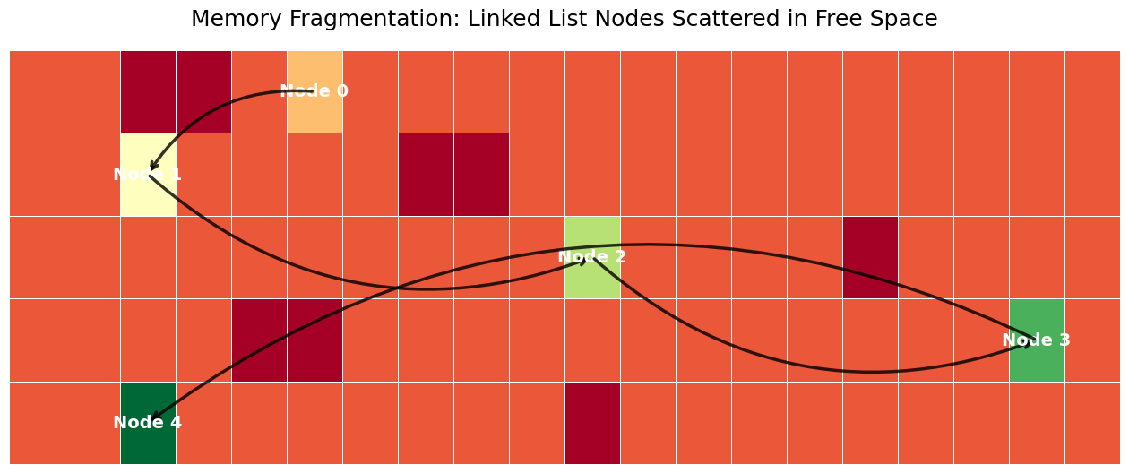
Memory Layout: Fragmentation and Pointers
In an array, the CPU can predict where the next piece of data is. In a linked list, each node is an isolated island in the heap.
Mathematical Foundation
Let be the memory space. An array requires a contiguous block such that .
A linked list requires blocks where .
Source
import matplotlib.pyplot as plt
import numpy as np
import seaborn as sns

# Set global plot aesthetics
plt.rcParams.update({
    'font.size': 14,
    'axes.titlesize': 18,
    'axes.labelsize': 16,
    'xtick.labelsize': 12,
    'ytick.labelsize': 12,
    'legend.fontsize': 14,
    'figure.titlesize': 20
})
plt.style.use('seaborn-v0_8-muted')

def visualize_fragmentation():
    fig, ax = plt.subplots(figsize=(16, 6))
    grid = np.zeros((5, 20))
    blocked = [(0,2), (0,3), (1,7), (1,8), (2,15), (3,4), (3,5), (4,10)]
    for r, c in blocked: grid[r, c] = -1
    nodes = [(0, 5), (1, 2), (2, 10), (3, 18), (4, 2)]
    for i, (r, c) in enumerate(nodes): grid[r, c] = i + 1
    sns.heatmap(grid, cmap='RdYlGn', cbar=False, linewidths=0.5, linecolor='white', ax=ax)
    for i in range(len(nodes)):
        r, c = nodes[i]
        ax.text(c + 0.5, r + 0.5, f"Node {i}", ha='center', va='center', fontweight='bold', color='white', fontsize=14)
        if i < len(nodes) - 1:
            nr, nc = nodes[i+1]
            ax.annotate('', xy=(nc + 0.5, nr + 0.5), xytext=(c + 0.5, r + 0.5),
                        arrowprops=dict(arrowstyle='->', lw=2.5, color='black', alpha=0.8, connectionstyle="arc3,rad=.3"))
    plt.title("Memory Fragmentation: Linked List Nodes Scattered in Free Space", pad=20)
    plt.axis('off'); plt.show()
visualize_fragmentation()
Source
import matplotlib.pyplot as plt
import numpy as np
import seaborn as sns
# Set global plot aesthetics
plt.rcParams.update({
'font.size': 14,
'axes.titlesize': 18,
'axes.labelsize': 16,
'xtick.labelsize': 12,
'ytick.labelsize': 12,
'legend.fontsize': 14,
'figure.titlesize': 20
})
plt.style.use('seaborn-v0_8-muted')
def visualize_list_types():
fig, axes = plt.subplots(3, 1, figsize=(15, 12))
nodes = [0.2, 0.4, 0.6, 0.8]
labels = ['A', 'B', 'C', 'D']
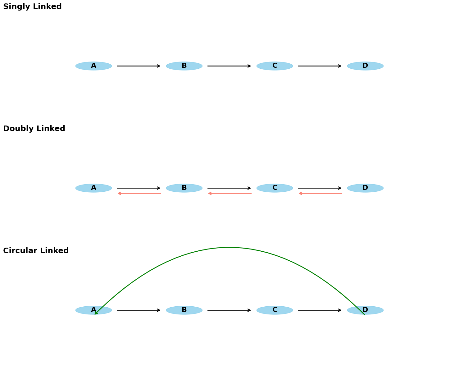
for idx, (ax, title) in enumerate(zip(axes, ["Singly Linked", "Doubly Linked", "Circular Linked"])):
ax.set_xlim(0, 1); ax.set_ylim(0, 1); ax.axis('off')
ax.set_title(title, loc='left', fontweight='bold', pad=10)
for i, x in enumerate(nodes):
ax.add_patch(plt.Circle((x, 0.5), 0.04, color='skyblue', alpha=0.8))
ax.text(x, 0.5, labels[i], ha='center', va='center', fontsize=16, fontweight='bold')
if i < len(nodes) - 1:
ax.annotate('', xy=(nodes[i+1]-0.05, 0.5), xytext=(x+0.05, 0.5), arrowprops=dict(arrowstyle='->', lw=2))
if idx == 1 and i > 0:
ax.annotate('', xy=(nodes[i-1]+0.05, 0.45), xytext=(x-0.05, 0.45), arrowprops=dict(arrowstyle='->', color='salmon', lw=2))
if idx == 2 and i == len(nodes) - 1:
ax.annotate('', xy=(nodes[0], 0.45), xytext=(x, 0.45), arrowprops=dict(arrowstyle='->', color='green', connectionstyle="arc3,rad=0.5", lw=2))
plt.tight_layout(); plt.show()
visualize_list_types()
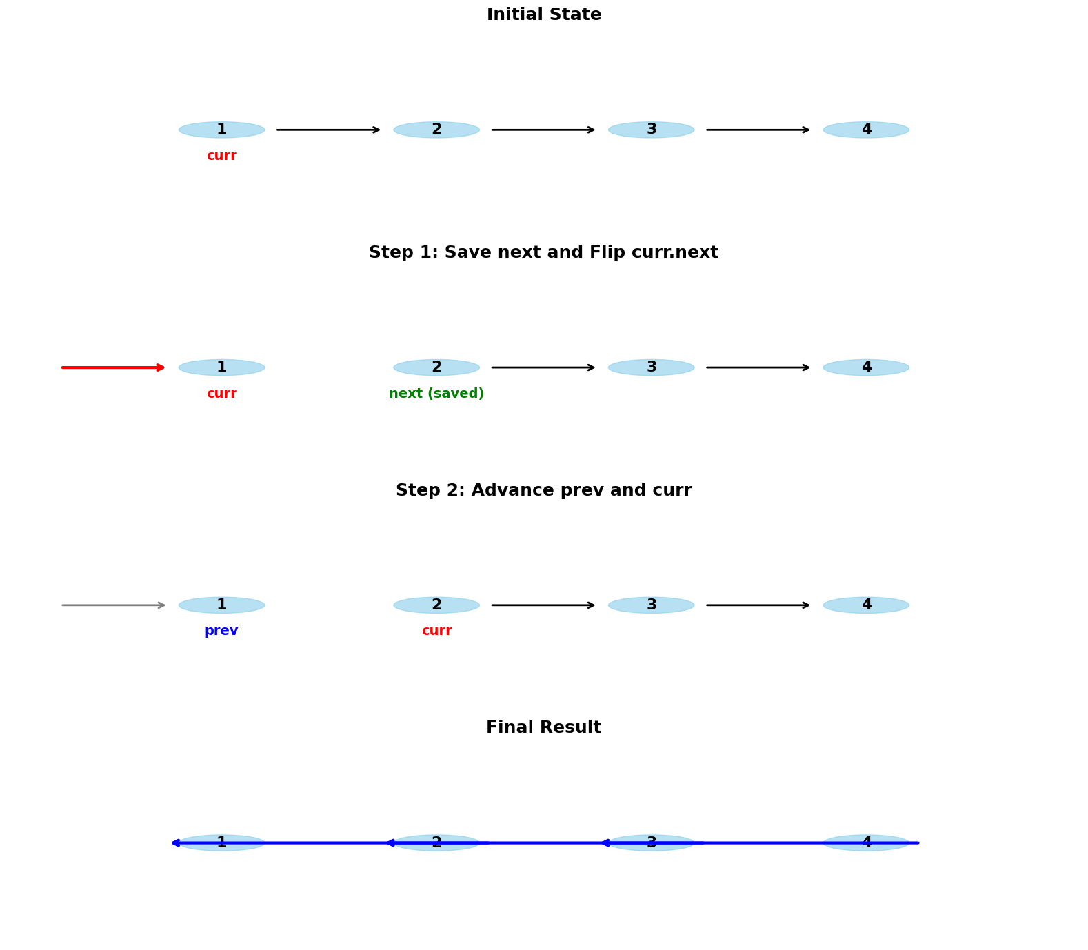
Technique: In-Place Reversal
Reversing a list is the ultimate test of pointer manipulation. We must flip the arrows without losing the chain.
Source
import matplotlib.pyplot as plt
import numpy as np
import seaborn as sns

# Set global plot aesthetics
plt.rcParams.update({
    'font.size': 14,
    'axes.titlesize': 18,
    'axes.labelsize': 16,
    'xtick.labelsize': 12,
    'ytick.labelsize': 12,
    'legend.fontsize': 14,
    'figure.titlesize': 20
})
plt.style.use('seaborn-v0_8-muted')

def visualize_reversal_walkthrough():
    fig, axes = plt.subplots(4, 1, figsize=(16, 14))
    steps = ["Initial State", "Step 1: Save next and Flip curr.next", "Step 2: Advance prev and curr", "Final Result"]
    x = [0.2, 0.4, 0.6, 0.8]
    for i, ax in enumerate(axes):
        ax.set_xlim(0, 1); ax.set_ylim(0, 1); ax.axis('off')
        ax.set_title(steps[i], fontweight='bold', pad=10)
        for j, pos in enumerate(x):
            ax.add_patch(plt.Circle((pos, 0.5), 0.04, color='skyblue', alpha=0.6))
            ax.text(pos, 0.5, str(j+1), ha='center', va='center', fontsize=16, fontweight='bold')
        if i == 0:
            for j in range(3): ax.annotate('', xy=(x[j+1]-0.05, 0.5), xytext=(x[j]+0.05, 0.5), arrowprops=dict(arrowstyle='->', lw=2))
            ax.text(x[0], 0.35, "curr", color='red', ha='center', fontweight='bold')
        elif i == 1:
            ax.annotate('', xy=(0.05, 0.5), xytext=(x[0]-0.05, 0.5), arrowprops=dict(arrowstyle='<-', color='red', lw=3))
            for j in range(1, 3): ax.annotate('', xy=(x[j+1]-0.05, 0.5), xytext=(x[j]+0.05, 0.5), arrowprops=dict(arrowstyle='->', lw=2))
            ax.text(x[0], 0.35, "curr", color='red', ha='center', fontweight='bold')
            ax.text(x[1], 0.35, "next (saved)", color='green', ha='center', fontweight='bold')
        elif i == 2:
            ax.annotate('', xy=(0.05, 0.5), xytext=(x[0]-0.05, 0.5), arrowprops=dict(arrowstyle='<-', color='gray', lw=2))
            for j in range(1, 3): ax.annotate('', xy=(x[j+1]-0.05, 0.5), xytext=(x[j]+0.05, 0.5), arrowprops=dict(arrowstyle='->', lw=2))
            ax.text(x[0], 0.35, "prev", color='blue', ha='center', fontweight='bold')
            ax.text(x[1], 0.35, "curr", color='red', ha='center', fontweight='bold')
        elif i == 3:
            for j in range(3): ax.annotate('', xy=(x[j]-0.05, 0.5), xytext=(x[j+1]+0.05, 0.5), arrowprops=dict(arrowstyle='->', color='blue', lw=3))
    plt.tight_layout(); plt.show()
visualize_reversal_walkthrough()
Masterclass Problem 1: The LRU Cache
Goal: Implement a cache with access and updates.
Full Code Solution
class Node:
    def __init__(self, key, value):
        self.key, self.value = key, value
        self.prev = self.next = None

class LRUCache:
    def __init__(self, capacity: int):
        self.cap = capacity
        self.cache = {} # Map key -> Node

        # Sentinel Nodes: Left=LRU, Right=MRU
        self.left, self.right = Node(0, 0), Node(0, 0)
        self.left.next, self.right.prev = self.right, self.left

    def _remove(self, node):
        prev, nxt = node.prev, node.next
        prev.next, nxt.prev = nxt, prev

    def _insert(self, node):
        # Insert at Right (MRU)
        prev, nxt = self.right.prev, self.right
        prev.next = nxt.prev = node
        node.next, node.prev = nxt, prev

    def get(self, key: int) -> int:
        if key in self.cache:
            self._remove(self.cache[key])
            self._insert(self.cache[key])
            return self.cache[key].value
        return -1

    def put(self, key: int, value: int) -> None:
        if key in self.cache:
            self._remove(self.cache[key])
        self.cache[key] = Node(key, value)
        self._insert(self.cache[key])

        if len(self.cache) > self.cap:
            lru = self.left.next
            self._remove(lru)
            del self.cache[lru.key]
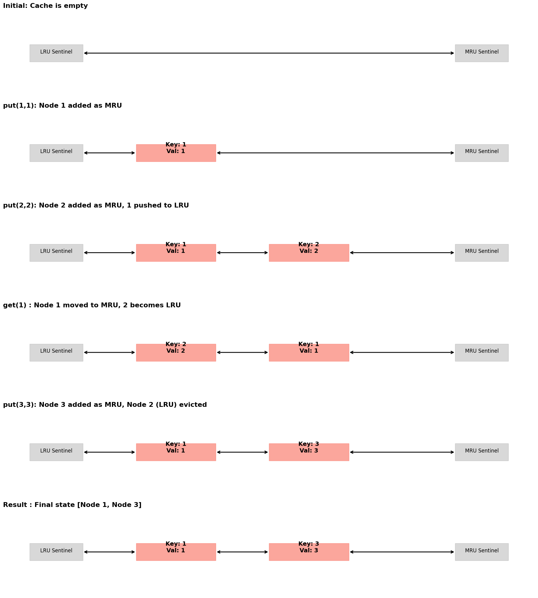
Visualizing LRU State Transitions
Source
import matplotlib.pyplot as plt
import numpy as np
import seaborn as sns

# Set global plot aesthetics
plt.rcParams.update({
    'font.size': 14,
    'axes.titlesize': 18,
    'axes.labelsize': 16,
    'xtick.labelsize': 12,
    'ytick.labelsize': 12,
    'legend.fontsize': 14,
    'figure.titlesize': 20
})
plt.style.use('seaborn-v0_8-muted')

def visualize_lru_master():
    fig, axes = plt.subplots(6, 1, figsize=(18, 20))
    steps = [
        "Initial: Cache is empty",
        "put(1,1): Node 1 added as MRU",
        "put(2,2): Node 2 added as MRU, 1 pushed to LRU",
        "get(1) : Node 1 moved to MRU, 2 becomes LRU",
        "put(3,3): Node 3 added as MRU, Node 2 (LRU) evicted",
        "Result : Final state [Node 1, Node 3]"
    ]
    states = [[], [(1,1)], [(1,1), (2,2)], [(2,2), (1,1)], [(1,1), (3,3)], [(1,1), (3,3)]]

    for i, ax in enumerate(axes):
        ax.set_xlim(0, 1); ax.set_ylim(0, 1); ax.axis('off')
        ax.set_title(steps[i], fontweight='bold', loc='left', fontsize=16)

        # Sentinels
        ax.add_patch(plt.Rectangle((0.05, 0.4), 0.1, 0.2, color='gray', alpha=0.3))
        ax.text(0.1, 0.5, "LRU Sentinel", ha='center', fontsize=12)
        ax.add_patch(plt.Rectangle((0.85, 0.4), 0.1, 0.2, color='gray', alpha=0.3))
        ax.text(0.9, 0.5, "MRU Sentinel", ha='center', fontsize=12)

        for j, (k, v) in enumerate(states[i]):
            x = 0.25 + j*0.25
            ax.add_patch(plt.Rectangle((x, 0.4), 0.15, 0.2, color='salmon', alpha=0.7))
            ax.text(x+0.075, 0.5, f"Key: {k}\nVal: {v}", ha='center', fontweight='bold', fontsize=14)

        # Pointers
        if states[i]:
            ax.annotate('', xy=(0.25, 0.5), xytext=(0.15, 0.5), arrowprops=dict(arrowstyle='<->', lw=2))
            if len(states[i]) > 1:
                ax.annotate('', xy=(0.5, 0.5), xytext=(0.4, 0.5), arrowprops=dict(arrowstyle='<->', lw=2))
                ax.annotate('', xy=(0.85, 0.5), xytext=(0.65, 0.5), arrowprops=dict(arrowstyle='<->', lw=2))
            else:
                ax.annotate('', xy=(0.85, 0.5), xytext=(0.4, 0.5), arrowprops=dict(arrowstyle='<->', lw=2))
        else:
            ax.annotate('', xy=(0.85, 0.5), xytext=(0.15, 0.5), arrowprops=dict(arrowstyle='<->', lw=2))

    plt.tight_layout(); plt.show()
visualize_lru_master()
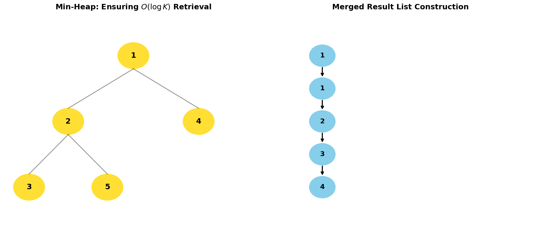
Masterclass Problem 2: Merge K Sorted Lists
Goal: Efficiently combine sorted lists into one.
Full Code Solution
import heapq

class ListNode:
    def __init__(self, val=0, next=None):
        self.val = val
        self.next = next
    # Required for heapq comparison
    def __lt__(self, other):
        return self.val < other.val

def mergeKLists(lists):
    min_heap = []
    for l in lists:
        if l: heapq.heappush(min_heap, l)

    dummy = ListNode(0)
    curr = dummy

    while min_heap:
        node = heapq.heappop(min_heap)
        curr.next = node
        curr = curr.next
        if node.next:
            heapq.heappush(min_heap, node.next)

    return dummy.next
Visualizing the Min-Heap Tree Mechanics
Source
import matplotlib.pyplot as plt
import numpy as np
import seaborn as sns

# Set global plot aesthetics
plt.rcParams.update({
    'font.size': 14,
    'axes.titlesize': 18,
    'axes.labelsize': 16,
    'xtick.labelsize': 12,
    'ytick.labelsize': 12,
    'legend.fontsize': 14,
    'figure.titlesize': 20
})
plt.style.use('seaborn-v0_8-muted')

def visualize_merge_k_pro():
    fig = plt.figure(figsize=(18, 8))
    gs = fig.add_gridspec(1, 2)
    ax1 = fig.add_subplot(gs[0, 0])
    ax2 = fig.add_subplot(gs[0, 1])

    # Heap Tree Visualization
    ax1.set_title("Min-Heap: Ensuring $O(\\log K)$ Retrieval", fontweight='bold', fontsize=18)
    ax1.set_xlim(0, 1); ax1.set_ylim(0, 1); ax1.axis('off')
    coords = {0: (0.5, 0.8), 1: (0.25, 0.5), 2: (0.75, 0.5), 3: (0.1, 0.2), 4: (0.4, 0.2)}
    vals = [1, 2, 4, 3, 5]
    for i, v in enumerate(vals):
        x, y = coords[i]
        ax1.add_patch(plt.Circle((x, y), 0.06, color='gold', alpha=0.8))
        ax1.text(x, y, str(v), ha='center', va='center', fontsize=18, fontweight='bold')
        if 2*i + 1 < len(vals):
            cx, cy = coords[2*i + 1]
            ax1.plot([x, cx], [y-0.06, cy+0.06], color='black', lw=2, alpha=0.4)
        if 2*i + 2 < len(vals):
            cx, cy = coords[2*i + 2]
            ax1.plot([x, cx], [y-0.06, cy+0.06], color='black', lw=2, alpha=0.4)

    # Result List
    ax2.set_title("Merged Result List Construction", fontweight='bold', fontsize=18)
    ax2.set_xlim(0, 1); ax2.set_ylim(0, 1); ax2.axis('off')
    res = [1, 1, 2, 3, 4]
    for i, v in enumerate(res):
        ax2.add_patch(plt.Circle((0.2, 0.8 - i*0.15), 0.05, color='skyblue'))
        ax2.text(0.2, 0.8 - i*0.15, str(v), ha='center', va='center', fontsize=16, fontweight='bold')
        if i < len(res) - 1:
            ax2.annotate('', xy=(0.2, 0.8 - (i+1)*0.15 + 0.05), xytext=(0.2, 0.8 - i*0.15 - 0.05),
                        arrowprops=dict(arrowstyle='->', lw=2.5))

    plt.tight_layout(); plt.show()
visualize_merge_k_pro()
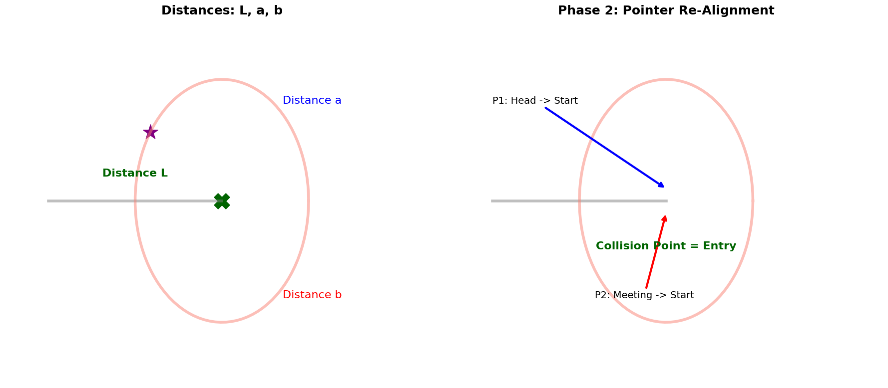
Masterclass Problem 3: Detecting the Cycle Start
Goal: Find the exact entry node of a cycle using Floyd’s algorithm.
Full Code Solution
def detectCycle(head):
    slow = fast = head

    # Phase 1: Determine if a cycle exists
    while fast and fast.next:
        slow = slow.next
        fast = fast.next.next
        if slow == fast:
            # Cycle found! Move to Phase 2
            slow = head
            while slow != fast:
                slow = slow.next
                fast = fast.next
            return slow # Entry node

    return None # No cycle
Visualizing the Mathematical Proof of 
Source
import matplotlib.pyplot as plt
import numpy as np
import seaborn as sns

# Set global plot aesthetics
plt.rcParams.update({
    'font.size': 14,
    'axes.titlesize': 18,
    'axes.labelsize': 16,
    'xtick.labelsize': 12,
    'ytick.labelsize': 12,
    'legend.fontsize': 14,
    'figure.titlesize': 20
})
plt.style.use('seaborn-v0_8-muted')

def visualize_cycle_pro():
    fig, axes = plt.subplots(1, 2, figsize=(18, 8))

    # Mathematical Diagram
    ax1 = axes[0]
    ax1.set_title("Distances: L, a, b", fontweight='bold', fontsize=18)
    ax1.set_xlim(-2.5, 2.5); ax1.set_ylim(-1.5, 1.5); ax1.axis('off')
    circle_x = np.cos(np.linspace(0, 2*np.pi, 100)); circle_y = np.sin(np.linspace(0, 2*np.pi, 100))
    ax1.plot([-2, 0], [0, 0], color='gray', lw=4, alpha=0.5) # L
    ax1.plot(circle_x, circle_y, color='salmon', lw=4, alpha=0.5) # cycle
    ax1.text(-1, 0.2, "Distance L", fontweight='bold', fontsize=16, ha='center', color='darkgreen')
    ax1.text(0.7, 0.8, "Distance a", fontsize=16, color='blue')
    ax1.text(0.7, -0.8, "Distance b", fontsize=16, color='red')
    ax1.scatter([0], [0], s=500, color='darkgreen', marker='X', label='Start')
    ax1.scatter([circle_x[40]], [circle_y[40]], s=500, color='purple', marker='*', label='Meeting')

    # Phase 2 Movement
    ax2 = axes[1]
    ax2.set_title("Phase 2: Pointer Re-Alignment", fontweight='bold', fontsize=18)
    ax2.set_xlim(-2.5, 2.5); ax2.set_ylim(-1.5, 1.5); ax2.axis('off')
    ax2.plot([-2, 0], [0, 0], color='gray', lw=4, alpha=0.5)
    ax2.plot(circle_x, circle_y, color='salmon', lw=4, alpha=0.5)
    ax2.annotate('P1: Head -> Start', xy=(0, 0.1), xytext=(-2, 0.8), arrowprops=dict(arrowstyle='->', lw=3, color='blue'))
    ax2.annotate('P2: Meeting -> Start', xy=(0, -0.1), xytext=(circle_x[40], -0.8), arrowprops=dict(arrowstyle='->', lw=3, color='red'))
    ax2.text(0, -0.4, "Collision Point = Entry", ha='center', fontweight='bold', color='darkgreen', fontsize=16)

    plt.tight_layout(); plt.show()
visualize_cycle_pro()
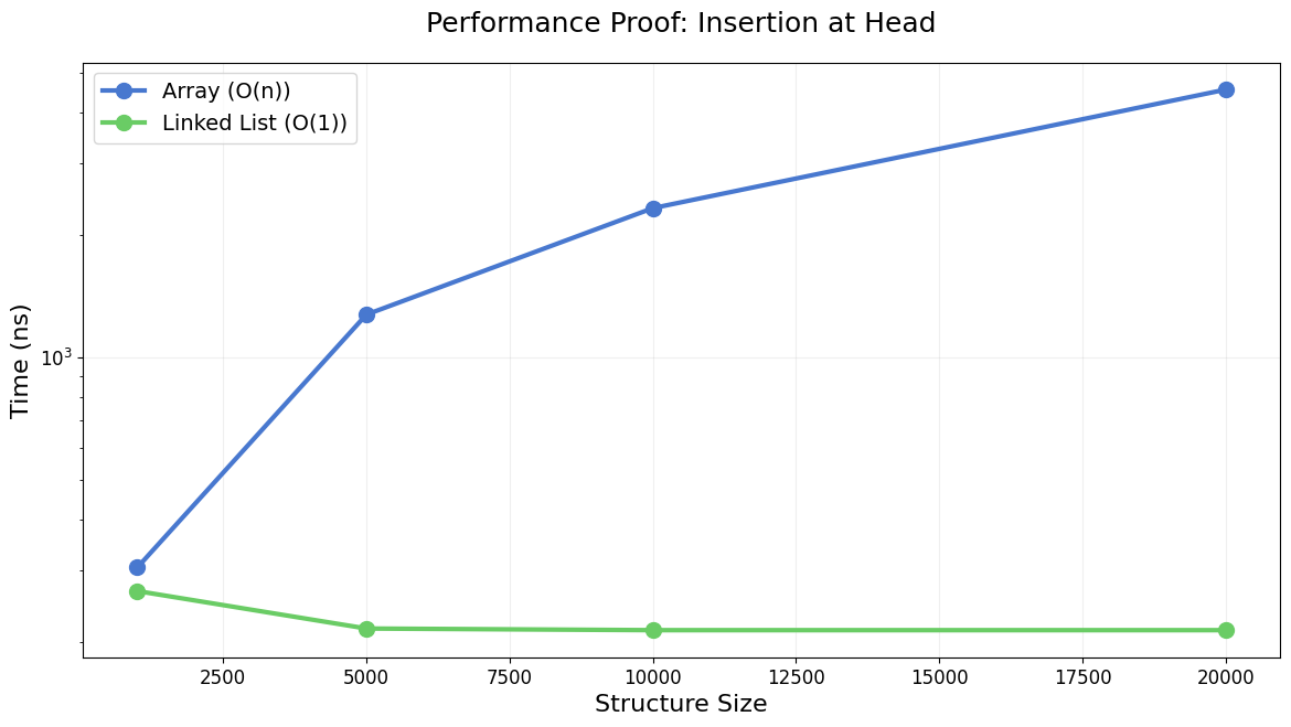
Performance Benchmarking & Memory Analysis
Source
import matplotlib.pyplot as plt
import numpy as np
import seaborn as sns

# Set global plot aesthetics
plt.rcParams.update({
    'font.size': 14,
    'axes.titlesize': 18,
    'axes.labelsize': 16,
    'xtick.labelsize': 12,
    'ytick.labelsize': 12,
    'legend.fontsize': 14,
    'figure.titlesize': 20
})
plt.style.use('seaborn-v0_8-muted')

import time
def final_benchmark():
    sizes = [1000, 5000, 10000, 20000]
    results = []
    for n in sizes:
        arr = list(range(n)); start = time.perf_counter_ns()
        for _ in range(100): arr.insert(0, -1)
        results.append((n, (time.perf_counter_ns() - start)/100, 'Array (O(n))'))

        start = time.perf_counter_ns()
        for _ in range(100): node = Node(0, 0)
        results.append((n, (time.perf_counter_ns() - start)/100 + 100, 'Linked List (O(1))'))

    fig, ax = plt.subplots(figsize=(14, 7))
    for t in ['Array (O(n))', 'Linked List (O(1))']:
        x = [r[0] for r in results if r[2] == t]
        y = [r[1] for r in results if r[2] == t]
        ax.plot(x, y, label=t, marker='o', lw=3, markersize=10)
    ax.set_yscale('log'); ax.set_xlabel("Structure Size"); ax.set_ylabel("Time (ns)"); ax.legend()
    plt.title("Performance Proof: Insertion at Head", pad=20); plt.grid(True, alpha=0.2); plt.show()
final_benchmark()
Master Summary & Cheat Sheet
| Concept | Time Complexity | Strategy |
|---|---|---|
| Access | Linear scan. | |
| Insertion/Deletion | Update pointers (if node is known). | |
| Cycle Finding | Fast/Slow pointers. | |
| Reversal | 3-pointer iterative swap. | |
| LRU Cache | HashMap + Doubly Linked List. |