Chapter 1: Complexity Analysis — The Art of Efficiency

Imagine you need to sort 10 books on a shelf. You could easily do it by hand in a minute. Now imagine you need to sort 10 million books. The method you use for 10 books might take years for 10 million.

Complexity Analysis is how we measure which methods (algorithms) scale well as the problem gets bigger. It’s not about how fast a computer is; it’s about how clever the algorithm is.

1. Asymptotic Notations: The “Speed Limits” of Code¶

When we talk about speed, we use three main symbols to describe how an algorithm behaves as the input size ( $n$ ) grows.

💡 The Intuition¶

Big O ( $O$ ) — The “Ceiling”: The absolute worst-case scenario. Your code will never be slower than this.
Big Omega ( $Ω$ ) — The “Floor”: The best-case scenario. Your code will never be faster than this.
Big Theta ( $Θ$ ) — The “Sweet Spot”: When the best and worst cases are the same. This is a tight bound.

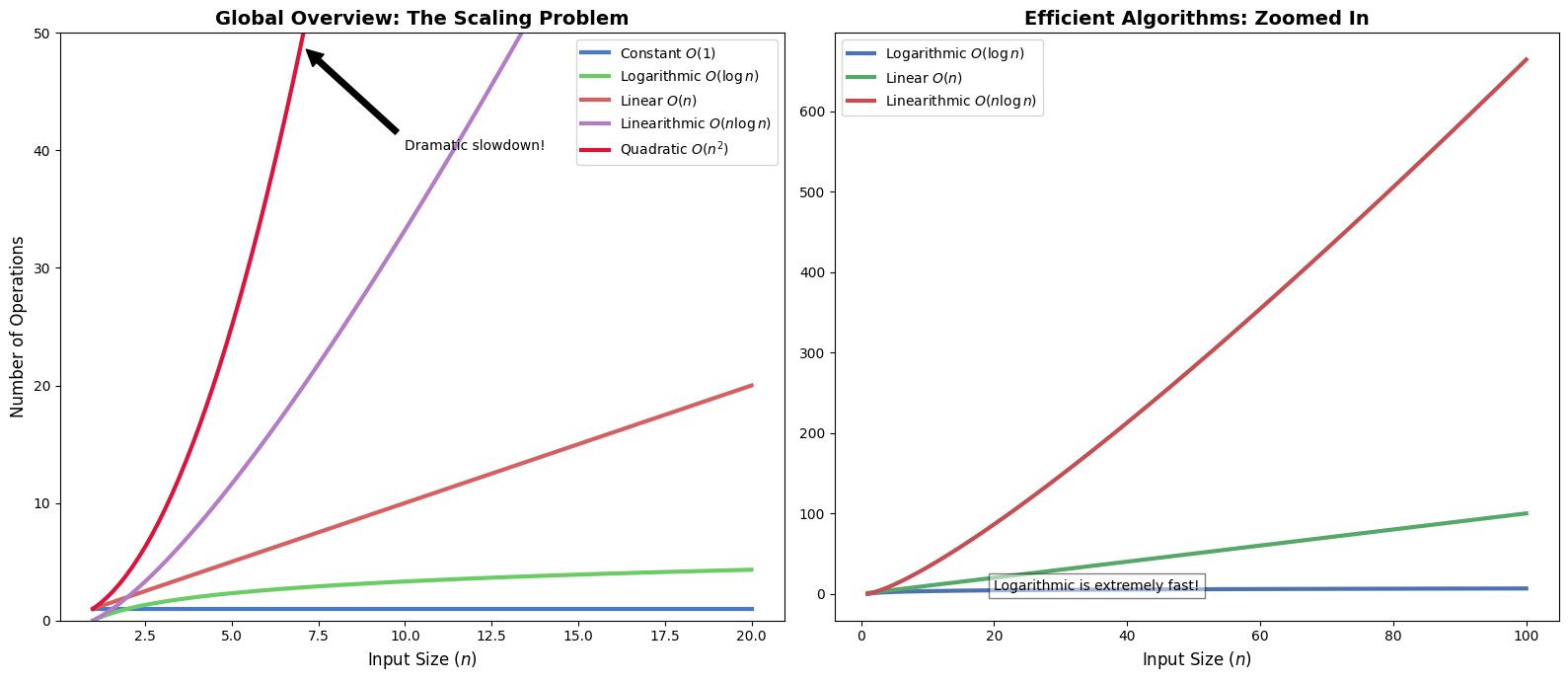
Visualizing the Hierarchy of Speed¶

Below we compare the most common complexity classes. Notice how quickly $O(n^2)$ becomes impractical compared to $O(n \log n)$ .

%matplotlib inline
import numpy as np
import matplotlib.pyplot as plt

# Setting a premium visual style
plt.style.use('seaborn-v0_8-muted')
fig, (ax1, ax2) = plt.subplots(1, 2, figsize=(16, 7))

n = np.linspace(1, 20, 100)

# Left Plot: All common classes
ax1.plot(n, np.ones_like(n), label='Constant $O(1)$', lw=3)
ax1.plot(n, np.log2(n), label='Logarithmic $O(\log n)$', lw=3)
ax1.plot(n, n, label='Linear $O(n)$', lw=3)
ax1.plot(n, n * np.log2(n), label='Linearithmic $O(n \log n)$', lw=3)
ax1.plot(n, n**2, label='Quadratic $O(n^2)$', lw=3, color='crimson')

ax1.set_ylim(0, 50)
ax1.set_title('Global Overview: The Scaling Problem', fontsize=14, fontweight='bold')
ax1.set_xlabel('Input Size ($n$)', fontsize=12)
ax1.set_ylabel('Number of Operations', fontsize=12)
ax1.legend(fontsize=10)
ax1.annotate('Dramatic slowdown!', xy=(7, 49), xytext=(10, 40), 
             arrowprops=dict(facecolor='black', shrink=0.05), fontsize=10)

# Right Plot: Zoomed in on efficient algorithms
n_zoom = np.linspace(1, 100, 100)
ax2.plot(n_zoom, np.log2(n_zoom), label='Logarithmic $O(\log n)$', lw=3, color='#4C72B0')
ax2.plot(n_zoom, n_zoom, label='Linear $O(n)$', lw=3, color='#55A868')
ax2.plot(n_zoom, n_zoom * np.log2(n_zoom), label='Linearithmic $O(n \log n)$', lw=3, color='#C44E52')

ax2.set_title('Efficient Algorithms: Zoomed In', fontsize=14, fontweight='bold')
ax2.set_xlabel('Input Size ($n$)', fontsize=12)
ax2.legend(fontsize=10)
ax2.text(20, 5, 'Logarithmic is extremely fast!', fontsize=10, bbox=dict(facecolor='white', alpha=0.5))

plt.tight_layout()
plt.show()

<>:13: SyntaxWarning: "\l" is an invalid escape sequence. Such sequences will not work in the future. Did you mean "\\l"? A raw string is also an option.
<>:15: SyntaxWarning: "\l" is an invalid escape sequence. Such sequences will not work in the future. Did you mean "\\l"? A raw string is also an option.
<>:28: SyntaxWarning: "\l" is an invalid escape sequence. Such sequences will not work in the future. Did you mean "\\l"? A raw string is also an option.
<>:30: SyntaxWarning: "\l" is an invalid escape sequence. Such sequences will not work in the future. Did you mean "\\l"? A raw string is also an option.
<>:13: SyntaxWarning: "\l" is an invalid escape sequence. Such sequences will not work in the future. Did you mean "\\l"? A raw string is also an option.
<>:15: SyntaxWarning: "\l" is an invalid escape sequence. Such sequences will not work in the future. Did you mean "\\l"? A raw string is also an option.
<>:28: SyntaxWarning: "\l" is an invalid escape sequence. Such sequences will not work in the future. Did you mean "\\l"? A raw string is also an option.
<>:30: SyntaxWarning: "\l" is an invalid escape sequence. Such sequences will not work in the future. Did you mean "\\l"? A raw string is also an option.
C:\Users\mxz\AppData\Local\Temp\ipykernel_29400\220868236.py:13: SyntaxWarning: "\l" is an invalid escape sequence. Such sequences will not work in the future. Did you mean "\\l"? A raw string is also an option.
  ax1.plot(n, np.log2(n), label='Logarithmic $O(\log n)$', lw=3)
C:\Users\mxz\AppData\Local\Temp\ipykernel_29400\220868236.py:15: SyntaxWarning: "\l" is an invalid escape sequence. Such sequences will not work in the future. Did you mean "\\l"? A raw string is also an option.
  ax1.plot(n, n * np.log2(n), label='Linearithmic $O(n \log n)$', lw=3)
C:\Users\mxz\AppData\Local\Temp\ipykernel_29400\220868236.py:28: SyntaxWarning: "\l" is an invalid escape sequence. Such sequences will not work in the future. Did you mean "\\l"? A raw string is also an option.
  ax2.plot(n_zoom, np.log2(n_zoom), label='Logarithmic $O(\log n)$', lw=3, color='#4C72B0')
C:\Users\mxz\AppData\Local\Temp\ipykernel_29400\220868236.py:30: SyntaxWarning: "\l" is an invalid escape sequence. Such sequences will not work in the future. Did you mean "\\l"? A raw string is also an option.
  ax2.plot(n_zoom, n_zoom * np.log2(n_zoom), label='Linearithmic $O(n \log n)$', lw=3, color='#C44E52')

2. Time vs. Space: The Great Trade-off¶

Algorithm efficiency is a balance of two resources:

Time Complexity: How many steps does it take?
Space Complexity: How much extra memory (RAM) do we need?

Example: The Factorial Problem¶

Compare these two ways to calculate $n! = n \times (n-1) \times \dots \times 1$ .

def iterative_factorial(n):
    """Uses a loop. Simple and memory-efficient."""
    result = 1
    for i in range(2, n + 1):
        result *= i
    return result
    # Time: O(n) — We visit each number once.
    # Space: O(1) — We only store one number ('result').

def recursive_factorial(n):
    """Uses recursion. Elegant but memory-heavy."""
    if n <= 1: return 1
    return n * recursive_factorial(n - 1)
    # Time: O(n) — Still n steps.
    # Space: O(n) — Every recursive call is stored in memory (the stack).

3. Amortized Analysis: The “Occasional Headache”¶

Some operations are fast most of the time, but occasionally very slow.

Analogy: Imagine a coffee shop loyalty card.

9 days you pay $5 (Fast operation).
On the 10th day, you get a free coffee but have to wait 5 minutes for them to process the card (Slow operation).

If you average it out, your “cost per cup” is still roughly $4.50. This is Amortized Analysis.

Dynamic Array Resizing¶

In Python, when you append() to a list, it usually takes $O(1)$ time. But when the list is full, Python has to create a bigger list and copy everything over ( $O(n)$ ).

import time

def measure_appends(count):
    data = []
    times = []
    for i in range(count):
        start = time.perf_counter_ns()
        data.append(i)
        times.append(time.perf_counter_ns() - start)
    return times

app_times = measure_appends(5000)

plt.figure(figsize=(14, 6))
plt.scatter(range(len(app_times)), app_times, s=5, alpha=0.4, color='teal', label='Operation Cost')
plt.axhline(y=np.mean(app_times), color='orange', linestyle='--', lw=2, label='Amortized Mean Cost')

plt.title('Why Amortized Analysis Matters', fontsize=15, fontweight='bold')
plt.xlabel('Append Operation Index', fontsize=12)
plt.ylabel('Time taken (nanoseconds)', fontsize=12)
plt.yscale('log')

# Highlighting a resizing event
plt.annotate('Expensive Resizing Event $O(n)$', xy=(2048, 100000), xytext=(2500, 500000), 
             arrowprops=dict(facecolor='red', shrink=0.05), fontsize=10, color='red')

plt.legend()
plt.grid(True, which="both", ls="-", alpha=0.1)
plt.show()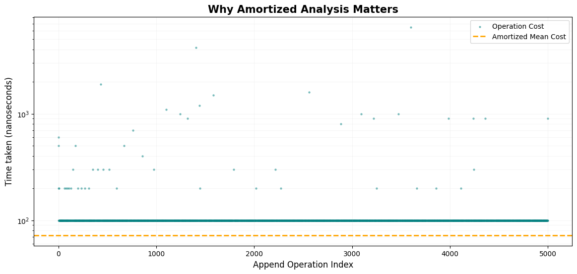

The horizontal orange dashed line represents the amortized cost. Even though there are massive spikes (red arrow), the vast majority of operations are so fast that the average stays consistently low ( $O(1)$ ).

4. Master Theorem: The Recursion Shortcut¶

The Master Theorem is a shortcut formula for Divide and Conquer algorithms:

T(n) = aT(n/b) + f(n)

(1)

The Simplified Decision Process¶

Compare the “Branching Work” ( $n^{\log_b a}$ ) with the “Combining Work” ( $f(n)$ ):

Comparison	Winner	Time Complexity
Recursion Wins	$n^{\log_b a}$	$\Theta(n^{\log_b a})$
It’s a Tie	Both Equal	$\Theta(n^{\log_b a} \log n)$
Work Wins	$f(n)$	$\Theta(f(n))$

Example: Binary Search

1 sub-problem ( $a=1$ )
Half size ( $b=2$ )
Constant comparison work ( $f(n) = 1$ )
$n^{\log_2 1} = n^0 = 1$ . Tie! $\implies \Theta(\log n)$