Chapter 3: Arrays and Strings

The Industrial Warehouse: Why Arrays Matter¶

Imagine an industrial warehouse with a row of numbered storage bins. Each bin is exactly the same size, and they are laid out in a perfectly straight line. If you know the bin number, you can walk directly to it in constant time, no matter how long the row is. This is the Static Array.

But what happens if you run out of bins? You can’t just squeeze a new one in the middleâ€”there’s no space. You have to rent a larger warehouse, move all your items one by one, and then add your new bin. This is the cost of Dynamic Array resizing.

In this chapter, we explore how this contiguous memory layout enables powerful patterns like Two Pointers and Sliding Windows, and why stringsâ€”despite their unique behavior in some languagesâ€”are fundamentally just specialized arrays of characters.

1. Memory Layout and Complexity¶

Arrays are stored in contiguous memory blocks. This means the memory address of any element $A[i]$ can be calculated using the base address $B$ , the index $i$ , and the size of each element $S$ :

\text{Address}(A[i]) = B + i \times S

(1)

This simple arithmetic is why array access is $O(1)$ .

Performance Proof: The Cost of Insertion¶

Let’s measure the difference between appending (which is usually $O(1)$ amortized) and inserting at the beginning (which is strictly $O(n)$ ).

import matplotlib.pyplot as plt
import numpy as np
import time

plt.style.use('seaborn-v0_8-muted')

def benchmark_arrays():
    sizes = [10**3, 5*10**3, 10**4, 2*10**4, 4*10**4]
    append_times = []
    insert_times = []
    
    for n in sizes:
        # Benchmark append
        start = time.perf_counter_ns()
        l1 = []
        for i in range(n):
            l1.append(i)
        append_times.append((time.perf_counter_ns() - start) / n)
        
        # Benchmark insert at 0
        start = time.perf_counter_ns()
        l2 = []
        for i in range(n):
            l2.insert(0, i)
        insert_times.append((time.perf_counter_ns() - start) / n)
        
    return sizes, append_times, insert_times

sizes, append_t, insert_t = benchmark_arrays()

fig, ax = plt.subplots(1, 2, figsize=(14, 5))

# Plot 1: Linear Scale
ax[0].plot(sizes, append_t, 'o-', label='Append (Amortized $O(1)$)')
ax[0].plot(sizes, insert_t, 's-', label='Insert at Start ($O(n)$)')
ax[0].set_title("Average Time per Operation (Linear Scale)")
ax[0].set_xlabel("Number of Elements (n)")
ax[0].set_ylabel("Time per op (ns)")
ax[0].legend()
ax[0].grid(True, alpha=0.3)

# Annotate the O(n) growth
ax[0].annotate('Linear growth: $O(n)$', xy=(sizes[-1], insert_t[-1]), xytext=(sizes[-2], insert_t[-1]*0.8),
            arrowprops=dict(facecolor='black', shrink=0.05, width=1, headwidth=5))

# Plot 2: Log-Log Scale (Big Picture)
ax[1].loglog(sizes, append_t, 'o-', label='Append')
ax[1].loglog(sizes, insert_t, 's-', label='Insert')
ax[1].set_title("Performance Scaling (Log-Log Scale)")
ax[1].set_xlabel("n")
ax[1].set_ylabel("Time per op (ns)")
ax[1].legend()
ax[1].grid(True, which="both", ls="-", alpha=0.2)

plt.tight_layout()
plt.show()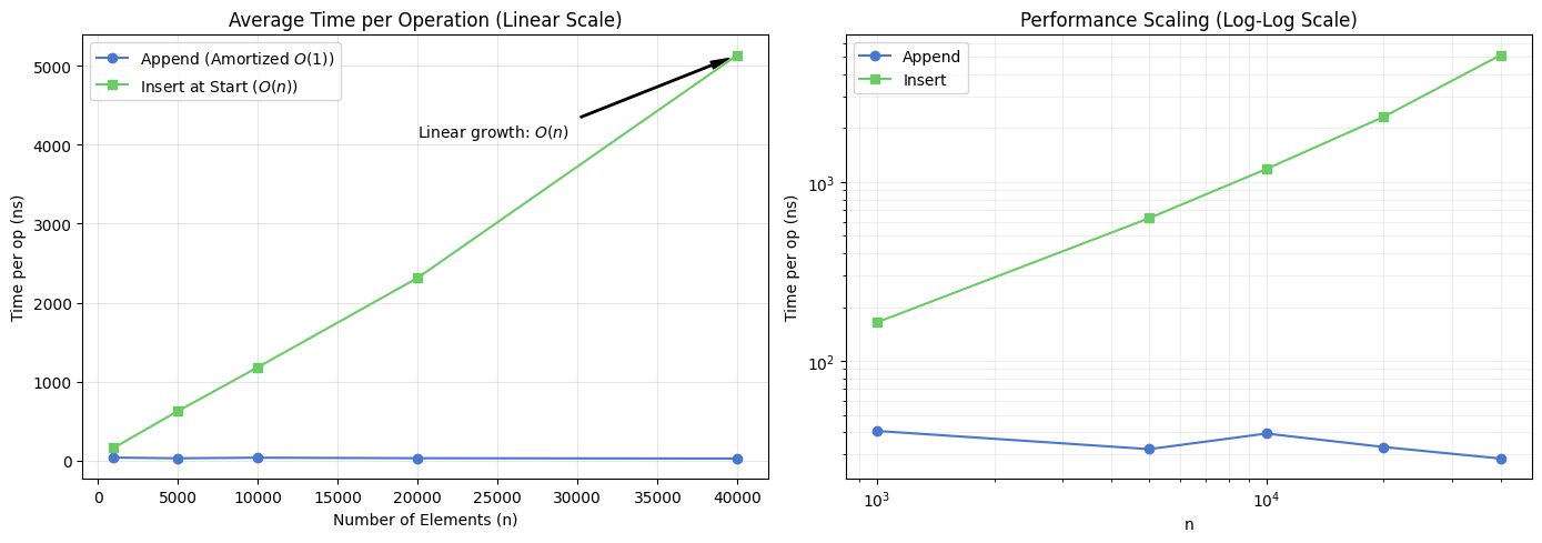

2. Deep Dive: The Two Pointers Pattern¶

Two pointers is a technique where two indices iterate through the data structure in tandem.

Problem: Two Sum II (Sorted Array)¶

Target: Find two indices such that $A[left] + A[right] = \text{Target}$ .

Intuition:¶

Since the array is sorted:

If our current sum is too small, we need to increase the sum. Moving the left pointer to the right ( $left++$ ) increases the value.
If our current sum is too large, we need to decrease the sum. Moving the right pointer to the left ( $right--$ ) decreases the value.

def two_sum_sorted(nums, target):
    left, right = 0, len(nums) - 1
    while left < right:
        current_sum = nums[left] + nums[right]
        if current_sum == target:
            return [left, right]
        elif current_sum < target:
            left += 1
        else:
            right -= 1
    return []

def visualize_two_sum(nums, target):
    left, right = 0, len(nums) - 1
    steps = []
    
    while left < right:
        current_sum = nums[left] + nums[right]
        steps.append((left, right, current_sum))
        if current_sum == target:
            break
        elif current_sum < target:
            left += 1
        else:
            right -= 1
            
    # Plotting the steps
    n_steps = len(steps)
    fig, axes = plt.subplots(n_steps, 1, figsize=(10, 2 * n_steps), sharex=True)
    if n_steps == 1: axes = [axes]
    
    for i, (l, r, s) in enumerate(steps):
        axes[i].bar(range(len(nums)), nums, color='lightgray', alpha=0.5)
        axes[i].bar([l, r], [nums[l], nums[r]], color=['skyblue', 'salmon'])
        axes[i].set_title(f"Step {i+1}: Sum = {nums[l]} + {nums[r]} = {s} ({'Too Small' if s < target else 'Too Large' if s > target else 'MATCH!'})")
        axes[i].set_xticks(range(len(nums)))
        axes[i].set_xticklabels(nums)
        
        # Add pointer labels
        axes[i].annotate('L', xy=(l, nums[l]), xytext=(l, nums[l]+5), ha='center', fontweight='bold')
        axes[i].annotate('R', xy=(r, nums[r]), xytext=(r, nums[r]+5), ha='center', fontweight='bold')

    plt.tight_layout()
    plt.show()

visualize_two_sum([2, 7, 11, 15, 18, 21], 26)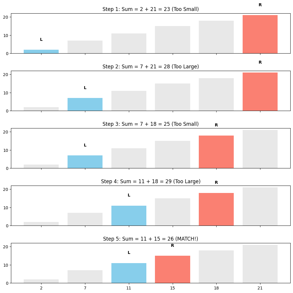

3. Deep Dive: Sliding Window (Dynamic)¶

The Sliding Window technique is used when we need to find a subarray that satisfies a specific condition.

Problem: Smallest Subarray with Sum $\ge S$ ¶

Goal: Find the minimum length of a contiguous subarray of which the sum $\ge S$ .

def min_subarray_len(s, nums):
    min_len = float('inf')
    current_sum = 0
    left = 0
    
    for right in range(len(nums)):
        current_sum += nums[right]
        while current_sum >= s:
            min_len = min(min_len, right - left + 1)
            current_sum -= nums[left]
            left += 1
            
    return min_len if min_len != float('inf') else 0

def visualize_sliding_window(nums, s):
    left = 0
    current_sum = 0
    history = []
    
    for right in range(len(nums)):
        current_sum += nums[right]
        history.append(('expand', left, right, current_sum))
        
        while current_sum >= s:
            history.append(('contract', left, right, current_sum))
            current_sum -= nums[left]
            left += 1
            
    # Visualize key moments
    events_to_show = history[:8]
    fig, axes = plt.subplots(len(events_to_show), 1, figsize=(10, 1.5 * len(events_to_show)))
    
    for i, (action, l, r, curr_s) in enumerate(events_to_show):
        colors = ['lightgray'] * len(nums)
        for idx in range(l, r + 1):
            colors[idx] = 'orange' if action == 'expand' else 'lightgreen'
            
        axes[i].bar(range(len(nums)), nums, color=colors)
        axes[i].set_title(f"Step {i+1}: {action.capitalize()} [Sum={curr_s}] Window indices: [{l}, {r}]")
        axes[i].set_xticks(range(len(nums)))
        axes[i].set_xticklabels(nums)

    plt.tight_layout()
    plt.show()

visualize_sliding_window([2, 3, 1, 2, 4, 3], 7)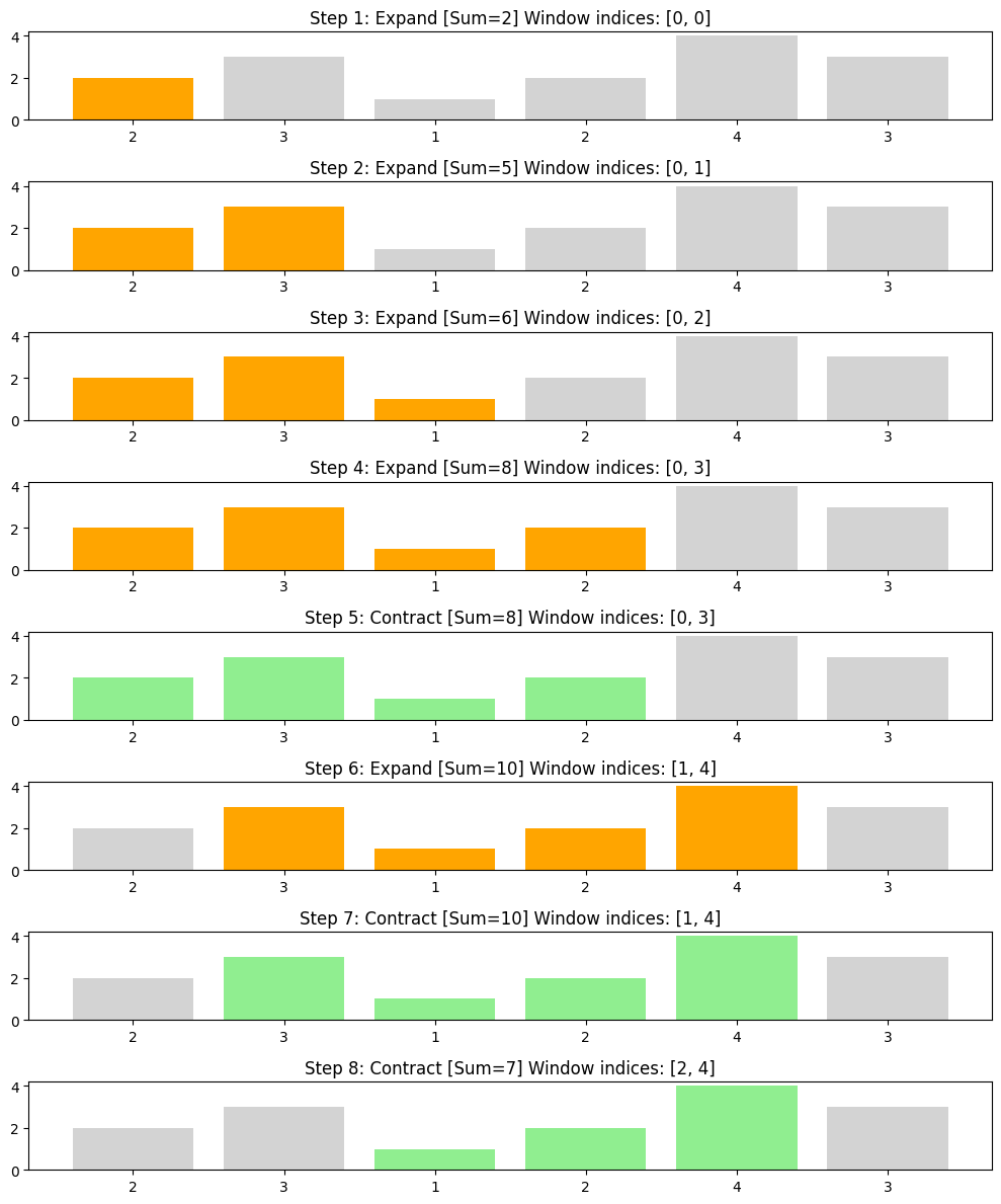

4. Specialized: Dutch National Flag (DNF)¶

def dutch_national_flag(nums):
    low, mid, high = 0, 0, len(nums) - 1
    while mid <= high:
        if nums[mid] == 0:
            nums[low], nums[mid] = nums[mid], nums[low]
            low += 1
            mid += 1
        elif nums[mid] == 1:
            mid += 1
        else:
            nums[mid], nums[high] = nums[high], nums[mid]
            high -= 1
    return nums

def visualize_dnf(nums):
    low, mid, high = 0, 0, len(nums) - 1
    snapshots = []
    snapshots.append((list(nums), low, mid, high))
    
    while mid <= high:
        if nums[mid] == 0:
            nums[low], nums[mid] = nums[mid], nums[low]
            low += 1
            mid += 1
        elif nums[mid] == 1:
            mid += 1
        else:
            nums[mid], nums[high] = nums[high], nums[mid]
            high -= 1
        snapshots.append((list(nums), low, mid, high))

    indices = [0, len(snapshots)//4, len(snapshots)//2, len(snapshots)-1]
    fig, axes = plt.subplots(4, 1, figsize=(10, 8))
    colors_map = {0: 'red', 1: 'white', 2: 'blue'}
    
    for i, snap_idx in enumerate(indices):
        arr, l, m, h = snapshots[snap_idx]
        bar_colors = [colors_map[x] for x in arr]
        axes[i].bar(range(len(arr)), [1]*len(arr), color=bar_colors, edgecolor='black')
        axes[i].set_title(f"Step {snap_idx}: low={l}, mid={m}, high={h}")
        axes[i].text(l, 1.1, 'L', ha='center', color='red', fontweight='bold')
        axes[i].text(m, 1.1, 'M', ha='center', color='black', fontweight='bold')
        axes[i].text(h, 1.1, 'H', ha='center', color='blue', fontweight='bold')
        axes[i].set_ylim(0, 1.5)
        axes[i].set_yticks([])

    plt.tight_layout()
    plt.show()

visualize_dnf([2, 0, 2, 1, 1, 0, 2, 1, 0])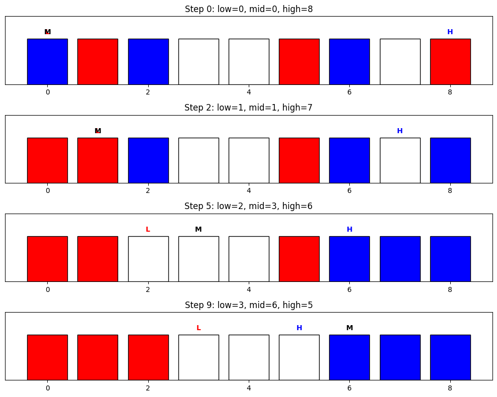

5. Specialized: Boyer-Moore Majority Vote¶

def get_majority_element(nums):
    candidate = None
    count = 0
    for x in nums:
        if count == 0:
            candidate = x
            count = 1
        elif x == candidate:
            count += 1
        else:
            count -= 1
    return candidate

def visualize_boyer_moore(nums):
    candidate = None
    count = 0
    history = []
    for x in nums:
        if count == 0: candidate = x; count = 1
        elif x == candidate: count += 1
        else: count -= 1
        history.append((candidate, count))
        
    fig, ax1 = plt.subplots(figsize=(10, 4))
    counts = [h[1] for h in history]
    candidates = [h[0] for h in history]
    ax1.step(range(len(nums)), counts, where='post', label='Current Count', color='purple', lw=2)
    ax1.set_xticks(range(len(nums)))
    ax1.set_xticklabels(nums)
    ax1.set_ylabel("Counter Value")
    ax1.set_title("Boyer-Moore: Counter Fluctuations")
    for i, cand in enumerate(candidates):
        ax1.text(i, counts[i] + 0.2, f"C={cand}", ha='center', fontsize=8)
    ax1.grid(True, alpha=0.3)
    plt.show()

visualize_boyer_moore([3, 3, 4, 2, 3, 3, 3, 1, 3])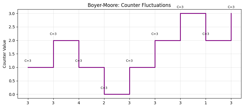

Complexity Table¶

Pattern	Time	Space	Core Idea
Two Pointers	$O(n)$	$O(1)$	Converging from ends (sorted) or parallel traversal.
Sliding Window	$O(n)$	$O(1)$	Maintaining a subset that moves or resized based on sum/frequency.
Prefix Sum	$O(n)$	$O(n)$	Pre-calculating cumulative sums for $O(1)$ range queries.
Boyer-Moore	$O(n)$	$O(1)$	Pairing up different elements to find a majority survivor.
DNF	$O(n)$	$O(1)$	3-way partitioning using three indices.

Interactive Pattern Recognition: “What should I use?”¶

Q: “Find the longest substring without repeating characters...” A: Sliding Window + Hash Map. Use the window to maintain uniqueness.

Q: “Find all pairs in a sorted array that sum to K...” A: Two Pointers. Move inwards based on current sum.

Q: “Sort an array of RGB colors represented by 0, 1, 2...” A: Dutch National Flag. 3-way partition in one pass.

Q: “Which element appears most often (if it’s > 50%)?” A: Boyer-Moore. The Survivor algorithm.